
This is a space where we go beyond luck and noise to uncover the repeatable logic behind extraordinary multibagger stock returns. I’ll be sharing my own ideas, frameworks, and investment theses here — built on first principles, research, and pattern recognition. The real power lies in collective insight. I’d love for you to contribute your own thoughts, questions, and theses.let’s decode the mechanics of multibaggers!
7 Likes
Understanding PE Through the EV, L Framework
1. Core Idea: PE = EV, L
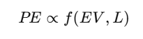
The Price/Earnings multiple (PE) a business deserves is not arbitrary. It’s a function of two things:
- Earnings Visibility (EV): How predictable and visible future earnings growth is.
- Longevity (L): How long those excess returns on capital can last before competition erodes them.
- So, in shorthand:
2. Earnings Visibility (EV)
Earnings visibility itself is not a single variable — it comes from three levers:
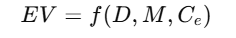
- M (Magnitude of TAM growth):
- How large the industry is and at what rate the total addressable market (TAM) is expanding.
- High M = big pie + fast growth → strong EV.
- Low M = small or slow pie → weak EV.
- D (Duration of Expansion cycle):
- How long the industry remains in the Expansion phase before hitting Peak → Recession → Recovery.
- Long D = multi-decade cycles (pharma, IT, paints).
- Short D = quick cycles (solar EPC booms, commodity upswings).
- Cₑ (Cyclicality within Expansion):
- Even during Expansion, earnings can be smooth or choppy.
- Low Cₑ = smooth expansion → high visibility → higher PE (Asian Paints, HDFC Bank).
- High Cₑ = choppy expansion → low visibility → capped PE (shrimp exports, mango pulp).
So, EV is strongest when:
- Magnitude is high (big fast-growing TAM),
- Duration is long (expansion phase lasts decades),
- Cyclicality is low (earnings are smooth and predictable).
3. Longevity (L)
Even if EV is strong, the market asks: can this last?
Formally, you can think of it as:
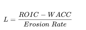
- ROIC – WACC: Is the business earning returns on invested capital above its cost of capital? The wider the spread, the stronger the competitive advantage.
- Erosion Rate: How quickly competition, technology, regulation, or customer behaviour erodes those returns.
- Low erosion → advantages last long → high Longevity.
- High erosion → advantages fade quickly → low Longevity.
So, Longevity captures the moat of the business.
Examples:
-
Nestlé India (brands, distribution, pricing power) → high L.
-
Shrimp exporter (commodity, replicable, disease/tariff shocks) → low L.
-
4. How This Maps to PE
-
High EV + High L → Very High PE
(Asian Paints, HDFC Bank, IT Services). -
High EV + Low L → Mid PE
(fast growers in commoditized industries, e.g. shrimp, pulp). -
Low EV + High L → Mid PE
(mature staples, cement; stable but slow). -
Low EV + Low L → Low PE
(cyclicals, commodity stocks).
5. Key Insight
- PE rerating happens when EV improves (longer, bigger, smoother cycle) and L strengthens (moat deepens).
- PE derating happens when EV collapses (cycle shortens or gets choppier) or L erodes (moat weakens).
17 Likes
Recipe for multibagger as per me -
- There are visible triggers for growth in company. Like company is expanding or can expand in new business or launching (can) new product and easily cross sell. These kind of companies don’t fall even in bad 1-2 quarter results.
- Company is in sector which has tailwinds for at least 3 years.
- Company market cap is very less than the TAM of the sector. TAM of the sector is expanding because of tailwinds.
- Retails share holding hasn’t increased. The less retail shareholding, better it is.
10 Likes
The Distribution Moat Mirage
A distribution moat by itself—say, wide dealer networks, warehouses, logistics fleets—does not guarantee defensibility. In fragmented markets like India, regional players can mirror distribution footprints quickly, sometimes even more efficiently because they’re hyper-local and lean.
The real strength comes when distribution layers with customer lock-in. Let’s unpack:
1. Switching Cost
If the product is tied into systems, training, or usage habits, the distributor becomes more than a transporter. For example:
- FMCG: Retailers often take credit terms, display support, and sales push. Switching isn’t just about stocking another brand—it means losing working capital float.
- Pharma: Doctors prescribing on long relationships; pharmacies rely on credit cycles and margin assurance.
2. Customer Stickiness
This arises when buyers prefer continuity because of trust, convenience, or bundled value. For instance:
- Paint dealers: Asian Paints dealers rarely switch to new entrants, not because distribution is unique, but because colour-mixing machines, dealer schemes, and customer recall are tied in.
- Beverages: Coca-Cola or Pepsi ensures chillers, signage, and festival promotions—distribution is inseparable from brand support.
3. Distribution as “Icing”
When switching cost and stickiness are in place, distribution ceases to be a commodity. It amplifies scale: a large distributor base ensures faster new launches, better credit rotation, and dominant shelf space. Without stickiness, however, it’s just a cost-heavy arm that competitors can copy.
distribution moat ≠ moat, unless coupled with lock-in or loyalty.
This raises an interesting thought experiment: in which industries in India today is distribution overvalued as a moat (e.g., packaged foods, cement) versus where it truly locks customers (e.g., paints, liquor)? That classification alone could tell you where incumbents’ valuations are fragile.
5 Likes
“Sideways Currents Ahead: Why Nifty May Deliver Only Average Returns”
As per Shankar Sharma’s Lake Return Theory
- Imagine a lake fed by multiple streams. Some years the streams gush, some years they trickle, but over decades the lake’s water level averages out.
- Applied to markets: Equity returns don’t follow a straight line. You get years of excess returns (floods) and years of poor returns (droughts), but in the long run they regress toward an average “water level.”
- For India, Sharma often pegs this long-term equity return mean around 12–15% CAGR.
- If you’ve just had a run of returns well above the average, expect mean reversion (sideways or weak returns). If returns have been below trend, the next block is more likely bullish.
So the “lake” = long-run return average; the “waves” = cycles of excess and scarcity.
Applying this to Nifty segmented data
Segmented Index Return exercise (1997–2025):
- 1-yr average: ~15.8%
- 3-yr average: ~12.3%
- 5-yr average: ~12.9%
That’s the “lake level” = low-to-mid teens.
Where are we now?
- 2017–22: 11.5% CAGR (5-yr)
- 2022–25 (so far): 12.3% CAGR (3-yr snapshot)
- These are bang in line with the long-term lake average (~12–13%).
- Contrast with the 2002–07 flood (41% CAGR) and 2007–12 drought (–0.8% CAGR). Today’s returns are not extreme at either end; they are “normal lake level.”
Projection for 2025–2030 using Lake Return logic
- Since current returns are already at the long-run average, there’s no pent-up “catch-up rally” like 2003, nor are we grotesquely over-extended like 2007.
- Valuations (Nifty TTM PE ~21.5) are above average, which historically leads to muted returns, not crashes, unless an external shock comes.
- That suggests the next 5 years will likely hover around the average CAGR (10–12%) → which is sideways in valuation terms, but mildly bullish in absolute terms.
Conclusion
- Not bullish super-cycle (like 2002–07).
- Not bearish washout (like 2007–12).
- Most probable: sideways-to-mildly bullish (10–12% CAGR over 2025–2030).
That’s Lake Return Theory in action: the lake has refilled to its normal level, so the next few years should see calm ripples, not floods or droughts.
1 Like
“The Variance Game: How Market Cycles Skew PE Rerating”
- PE Rerating is not absolute; it is market-contextual.
- The same fundamentals (sales growth, OPM expansion) can lead to very different PE outcomes depending on whether the broader market is in bull, sideways, or bear phase.
- Which means: if the lake ahead is shallow (sideways market), the PE rerating engine has much less fuel.
Framing this as a Concept
Let’s call it the “Market-Multiplier Dependence” (MMD) effect.
-
Earnings Growth = Company’s internal engine (sales + OPM).
-
PE Rerating = Market’s external multiplier.
-
The multiplier itself is cyclical.
-
In bull markets, PE can expand 2–3x → outsized returns.
-
In sideways markets, PE expansion is capped → only earnings growth drives returns.
-
In bear markets, PE can contract → earnings growth may be fully offset.
Linking to Lake Return Theory (Shankar Sharma’s analogy)
- If past 5-year returns are above average, the market lake is “full” → PE contraction/sideways ahead.
- If past returns are below average, the lake is “empty” → scope for rerating.
- ahead of us is a sideways lake → so depending on PE rerating is dangerous.
Implication for Investing Strategy
- In bull phases → chase high PE rerating candidates
- In sideways phases → focus on Earnings Compounding stories where Sales × OPM alone can deliver 15–20% CAGR
- In bear phases → margin of safety (MOS) + cash flow resilience become more important than growth.
3 Likes
Recipe for multibagger as per me -
Identify a company which is facing short term tailwinds with margin compression and having more than 1.5x gross block growth and also at a reasonable valuations
becos most of the time when margin compress and pat decreases, the p/e multiple spikes.
if we able to find the company with these things..
i’m sure we can make 2-3x return in 2-3 years but its not simple
Returns are made of 3 components -
Dividend + EPS growth + Valuation rerating
during capex, co generally don’t give dividend so we can ignore it.
now suppose we identify a compay with 5cr PAT (and that is of low margin suppose of 5%) with P/E multiple of 20… its a 100cr mcap co.
and after 2-3 quarter, things start improving, sales grows to 200cr in 2 year with margin of 15-16% then PAT is of 30cr
and if this happens, we will see the P/E rerating also like to 40-50 times of earnings
30*40 = 1200cr
its 12 bagger in 2-3 years
but these things looks good on spreadsheets only, identifying these stocks and having conviction to ride till 12 bagger with good position sizing matters alot.
Ex. Guj themis biosyn
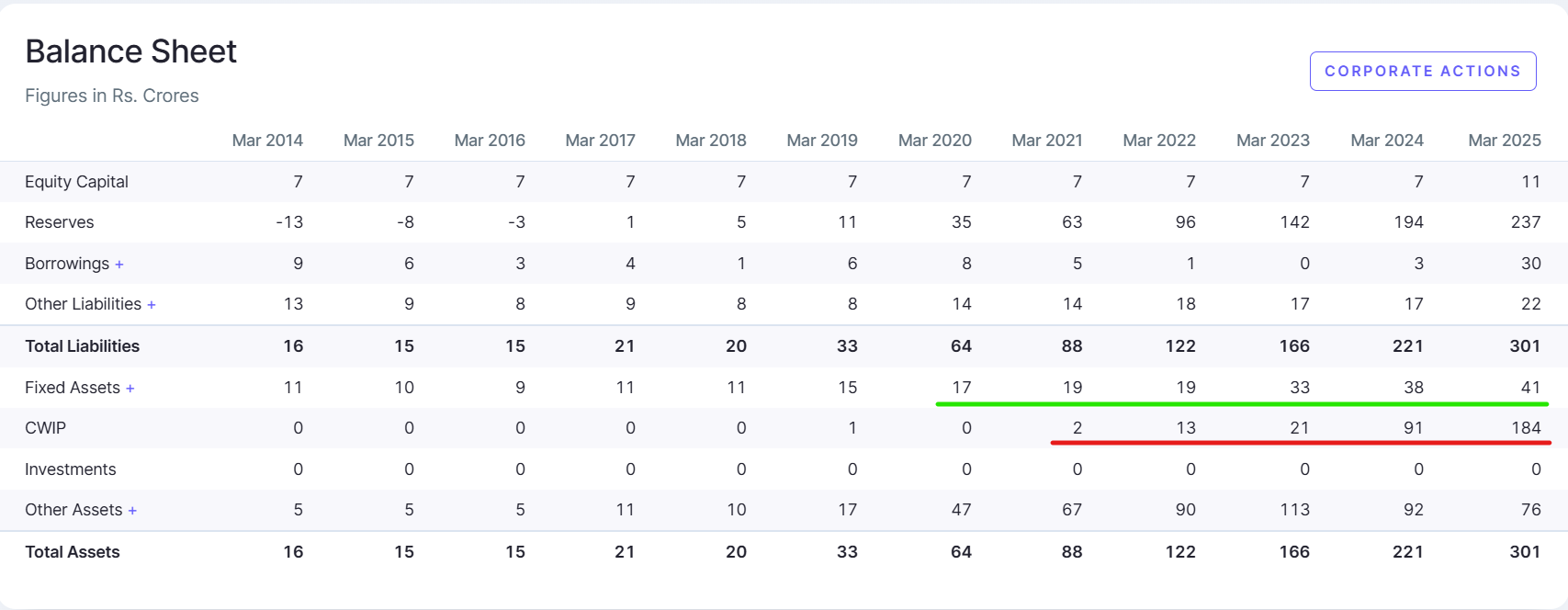
I identified the stock in 2021 when stock has fixed asset of 19cr and they are doing big capex
in FY21, co reported 90cr sales with 30cr of PAT with P/E multiple of 10-11 times
Co done capex in 2022 and still going under big changes
FY25 sales 151cr with PAT of 49cr with P/E multiple rerated to 97 times
FY25 fixed asset is 41cr and 184cr CWIP
stock rose from 30 levels to 400 levels
Mistake I did -
not giving sufficient allocation to the stock, initially it was of 2-3% of my portfolio, I should have given it 8-9% allocation
and currently its of 4-5% of portfolio…
still thinking about trimming becos capex commission is getting delayed, management stopped doing concalls, and expensive valuations.
7 Likes
Thank you for the brilliant insight. The combination of depressed operating margins alongside a substantial rise in gross block is a powerful observation. Looking forward to more of your posts. ![]()
1 Like
Sir the level of PE rerating which has taken place in Covid Bull Run is something we won’t see in the coming years. If you look closely PE shot up from level of 15-20 to 60-70 in Gujarat Themis Biosyn.
1 Like
yes I agree on that, that is the main reason for which i m not increasing my allocation right now.
I’m waiting for EPS expansion now, if this happens in this FY, then only I will increase the allocation.
“The Leaking Moat Problem”
- Moat Deepening = Valuation Sustenance.
- If management does not continuously reinforce or widen the moat, the inevitable force of competition erodes advantage.
- Even if topline grows and business looks “good,” the market will pre-empt margin erosion and derate the PE multiple.
Let’s shape this into a concept
We can call it:
“The Moat–Multiple Nexus”
Core principle: Sustainable valuation multiples are directly proportional to management’s ability to deepen moats faster than competitors can replicate advantages.
Mechanics
- Phase 1: Discovery & Growth
- New product/segment → high growth, PE rerating.
- Moat is “thin,” but growth hides vulnerability.
- Phase 2: Competition Enters
- Rivals replicate.
- If management doesn’t invest in deeper moat (brand, distribution, IP, switching costs, network effects) → margins compress.
- Phase 3: Market Adjusts
- PE derating begins before earnings fall, because markets discount future margin pressure.
- Phase 4: Survivors
- Companies that keep layering moats → maintain or even expand multiples.
- Others stagnate
Equation form
PE Sustenance = f(Moat Deepening Rate – Competitive Replication Rate)
- If Moat Deepening > Competition, PE stable/expands.
- If Moat Deepening < Competition, PE derates regardless of earnings growth.
Why this matters
It closes the loop:
- Lake Return Theory → tells you what the market cycle allows.
- Mirage of Multiples → PE rerating is phase-dependent.
- Moat–Multiple Nexus → even in a bull lake, if moat isn’t deepened, PE rerates briefly then derates structurally.
3 Likes
Thanks for sharing, very clear and simple explanation.
1 Like