
No. I use the current growth rate of the economy (Or lower) as the Terminal Growth Rate. Prof. Aswath Damodaran uses the Risk-free Rate as the upper bound, so my model adapts his ideas. Of course, this is iffy, but the concept being if a company grows at a rate higher than the GDP growth rate, given enough time, the company will become bigger than the country itself. That is an absurd picture. So, no company can grow faster than the economy (Here–7%–your proposition) “forever”. The Inflation Rate in an economy is another upper limit that can be used.
I’m not sure what you mean wrt Discounting Rate. The mode has 4 Options: Risk-free Rate, CAPM Beta-based WACC, Bottom-up Beta-based WACC and Opportunity Cost, which is an option that allows you to enter any figure (I just made the figure 50% higher than the Risk-free Rate by default - it can be changed manually).
I have to note here that the model is a combination of numbers and stories. It also has a Diagnosis tool in order to check if the estimates are within bounds. Of course, a Valuation exercise is no exam and nobody is going to grade the assumptions. But by forcing the investor to be objective about the numbers, it appeals to their logical mind. This is far better than typing out a bunch of numbers and have another number thrown out, with no idea of what happened in the middle or if that makes logical sense.
It is almost impossible to know what will happen to a company tomorrow, let alone 10 years from now. But an investor needs baseline assumptions in order to anchor his purchase price. All Valuation models have these assumptions. Even if you take the best model created by the biggest investments bank in the world, you’d still see a list of assumptions that need to be doled out. As Warren Buffet puts it, “It’s better to be grossly right than to be precisely wrong.” I’d already mentioned the caveats of the DCF and how to make up for them (Very conservative assumptions and a Margin of Safety).
As I mentioned earlier somewhere, I don’t believe in Betas. Volatility does not represent Risk. Volatility is Risk for a trader, not an investor. And Risk is not and never should be common for every investor (As is the case with Beta-based WACC calculations). Risk differs from person to person. Only that specific individual can come up with an appropriate Discounting Rate representing that Risk. You may buy a stock at Rs. 150 and I may buy it at Rs. 200 and we’d both be correct. Richard Thaler won the Nobel Prize because he was able to prove that different investors have different Risk tendencies towards different types of investments. Betas don’t allow for all this and that’s wrong.
But I get the general question you are trying to ask: With so many assumptions and some of them very sensitive to the value, how can we be sure that we’re not wrong? We can’t be exactly right, but “grossly right”. How do we do that? By accounting for the elephant in the room – randomness. No assumption in any valuation model is set in stone. It is subject to a lot of variability over time. So, a better way to be sure about the Value is to do a Monte Carlo Simulation (Link to a MCS Excel Add-in), using a variation limit, say 25%. In Excel, this would be “=RANDBETWEEN(-25,25)/100”
Again, going with the same KRBL valuation, I am applying a 25% variation to the following:
- Sales Growth: Randomized between 3.75% and 6.25% (Careful not to exceed the upper limit of Risk-free Rate)
- Target OPM: Randomized between 15% and 25%
- Depreciation/Sales: Randomized between 1.56% and 2.61%
- Capital Turnover: Randomized between 0.87 and 1.44
- Discounting Rate: Randomized between 7.29% and 11.94% (I put an IF condition, limiting downside of Discounting Rate to Risk-free Rate, so if a randomized event is 9.55%*(1-0.25) = 7.16%, the model will return 7.29% instead)
This is how the output looks like:
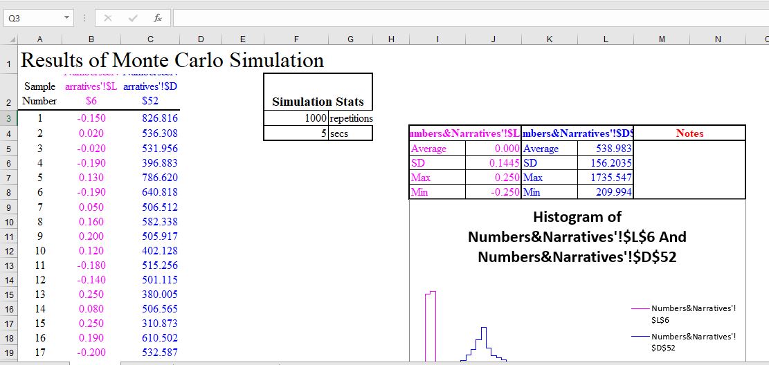
After some Excel maneuvering, you can present this data in a neat diagram:
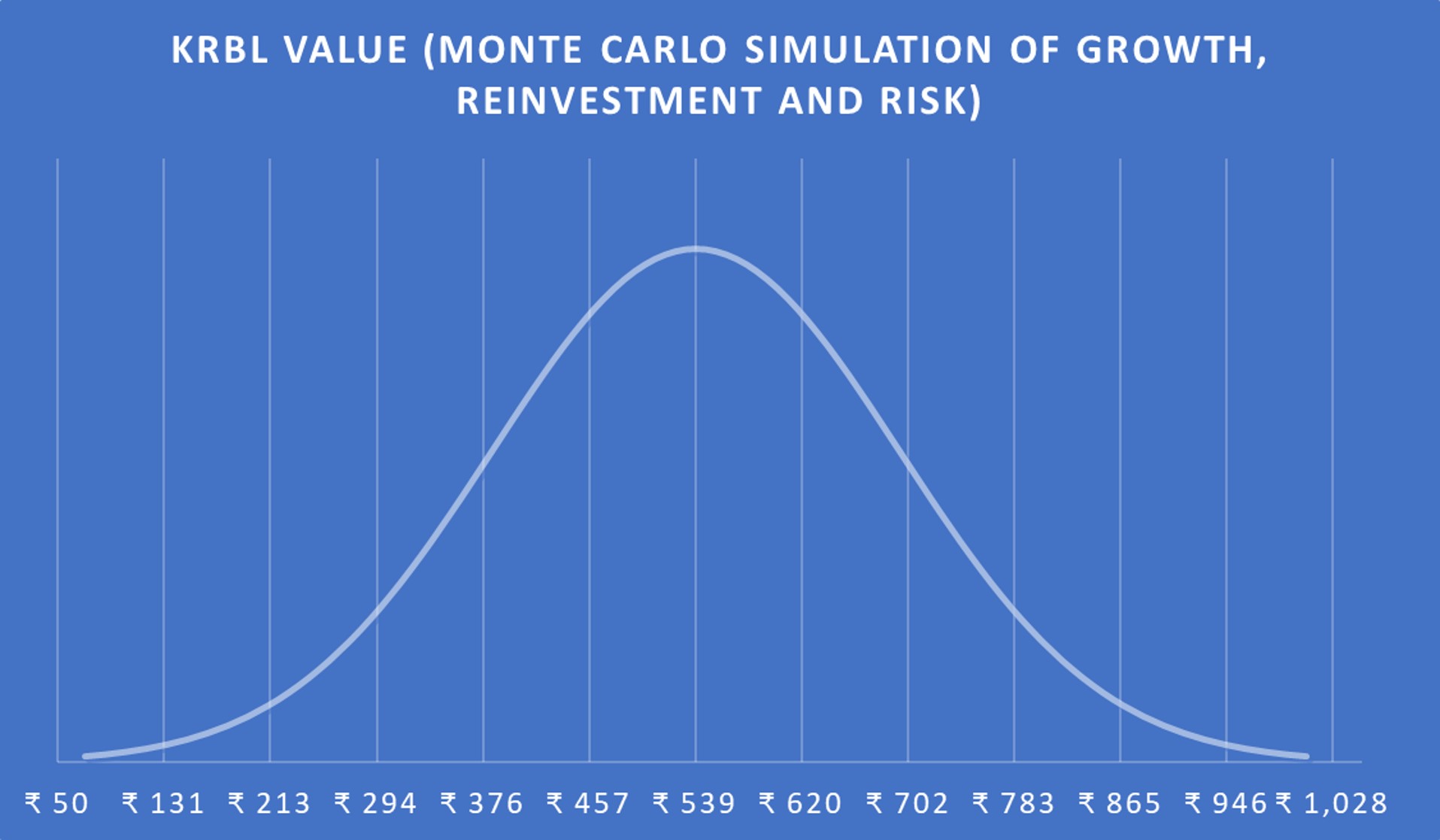
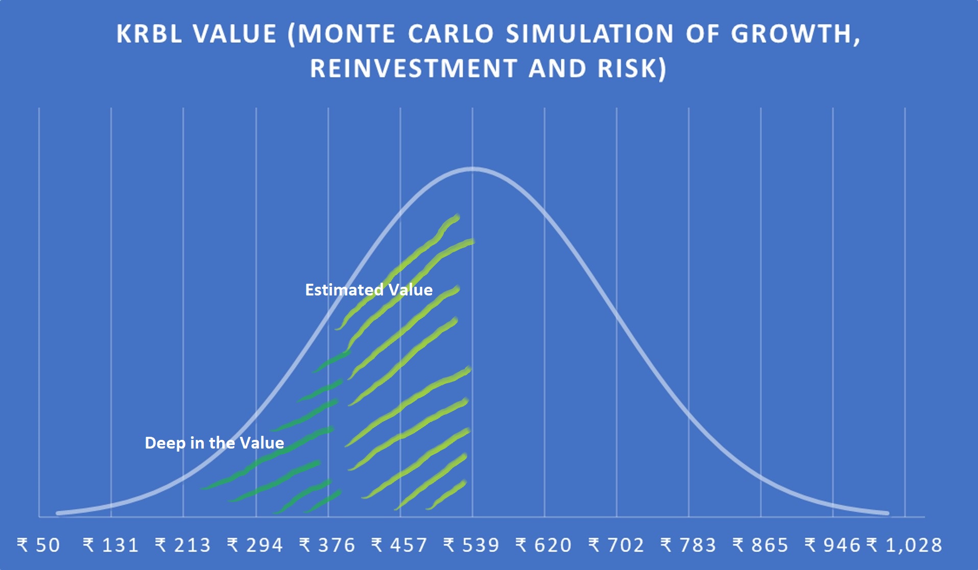
If you have an understanding of Probability, the above diagram simply shows that the Values at the far end of the graph (Rs. 50-Rs.294 or Rs. 783-Rs.1028) are most definitely incorrect. The ones inside are far better estimates, ranging from Rs. 294 to Rs. 783. Out of those, Rs. 539 is the most likely estimate. This is how you can eliminate the risk of randomness in a DCF (Or any model, really).
I thought long and hard about including a Monte Carlo Simulation tool in the model, but decided against it. The aim of the model is to be a simple tool to enable an investor to anchor his price to a probable value, not one with clunky formulas running into pages. If you have a good understanding of how to run a Monte Carlo Simulation and convert it into a Normal graph, feel free to use the link I have provided above for the MCS Excel Add-in. If you don’t, no worries. Using the model, keeping in mind its constraints would suffice too.